HKUST CSIT5401 Recognition System lecture notes 6. 识别系统复习笔记。
Vehicle recognition, including detection, tracking and identification, has been a research topic among automotive manufacturers, suppliers and universities for enhancing road safety.
For example, the ARGO project, started in 1996 at the University of Parma and the University of Pavia, Italy, is aimed at developing a system for improving road safety by controlling and supervising the driver activity.
- Lane Detection
- Vehicle Detection based on Symmetry
- Visual Saliency For Detection and Tracking
- Application Examples
Lane Detection
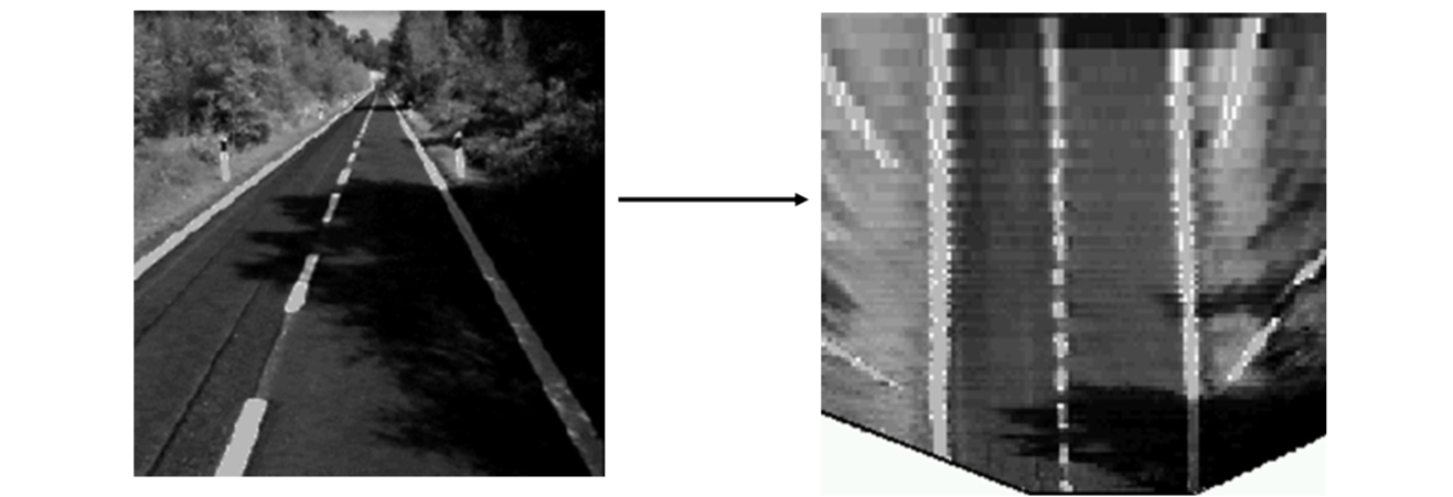
For vehicle detection and tracking and intelligent transportation systems, lane marking detection is one of the key steps. Lane markings can be detected based on the camera inverse perspective mapping (IPM) and the assumption that the lane markings are represented by almost vertical bright lines of constant width, surrounded by a darker background.
The lanes can then be detected by using the camera inverse perspective mapping (IPM) and the Canny edge detector.
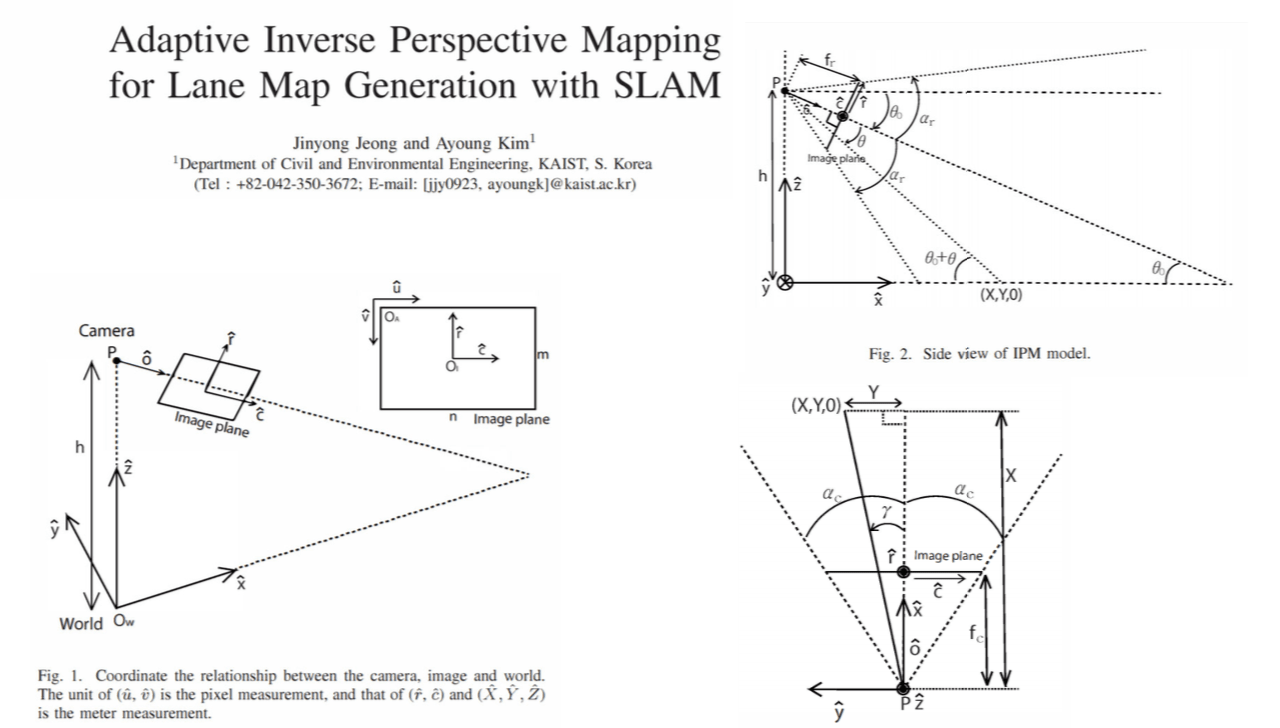
Inverse perspective mapping
Canny edge detector
Canny edge detector is one of the most popular detectors of edge pixels. The edge detection process serves to simplify the analysis of images by drastically reducing the amount of data to be processed, while at the same time preserving useful structural information about object boundaries.
There are three common criteria relevant to edge detector performance.
- It is important that edges that occur in the image should not be missed and that there be no spurious responses.
- The edge points should be well localized. That is, the distance between the points marked by the detector and the true edge center should be minimized.
- The last requirement is to circumvent the possibility of multiple responses to a single edge.
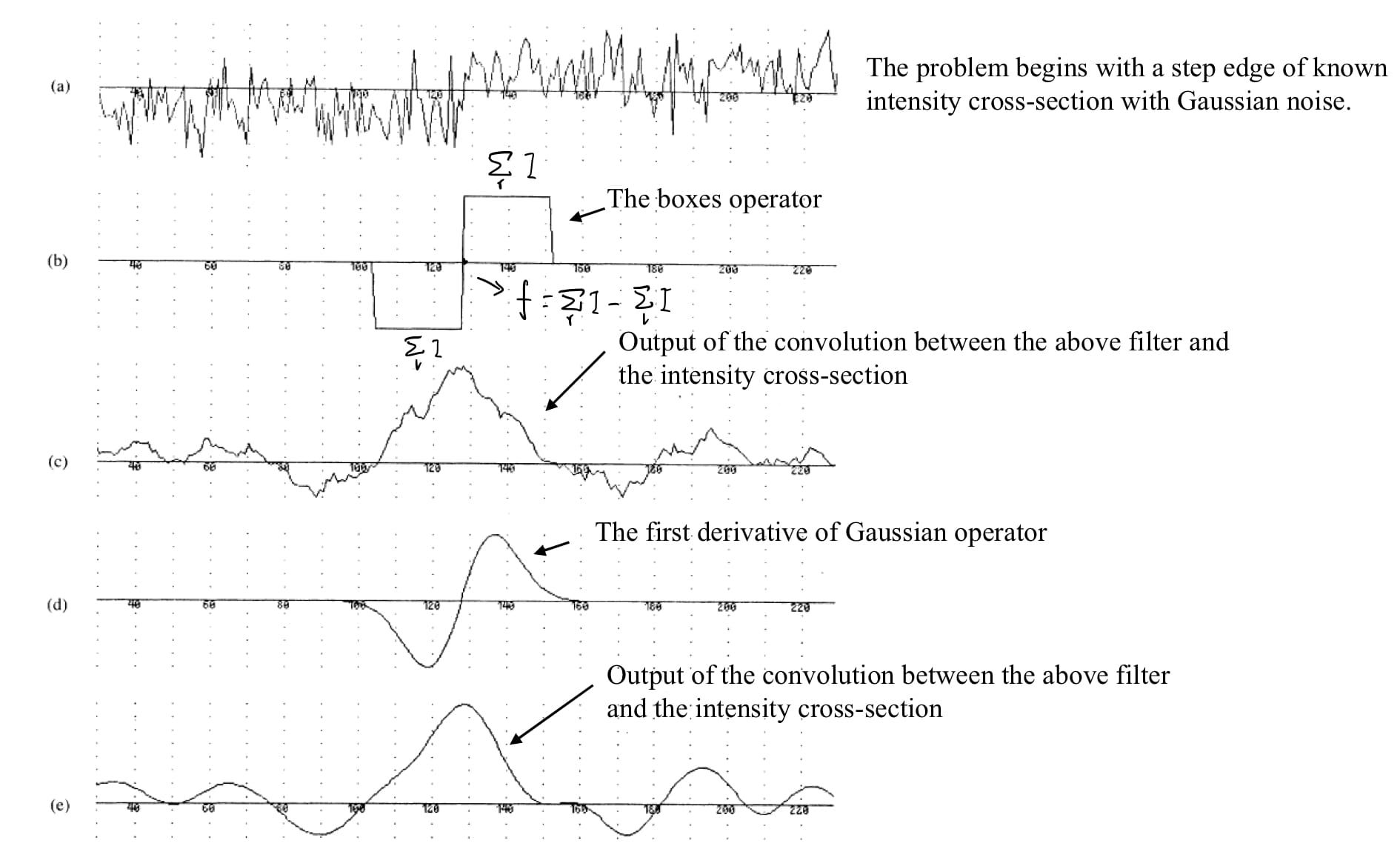
In the figure above, (a) is a noisy step edge; (b) is a difference of boxes operator; (c) is the output of filtering by box operator; (d) is the first derivative of Gaussian operator; and (e) is the first derivative of Gaussian applied to the edge.
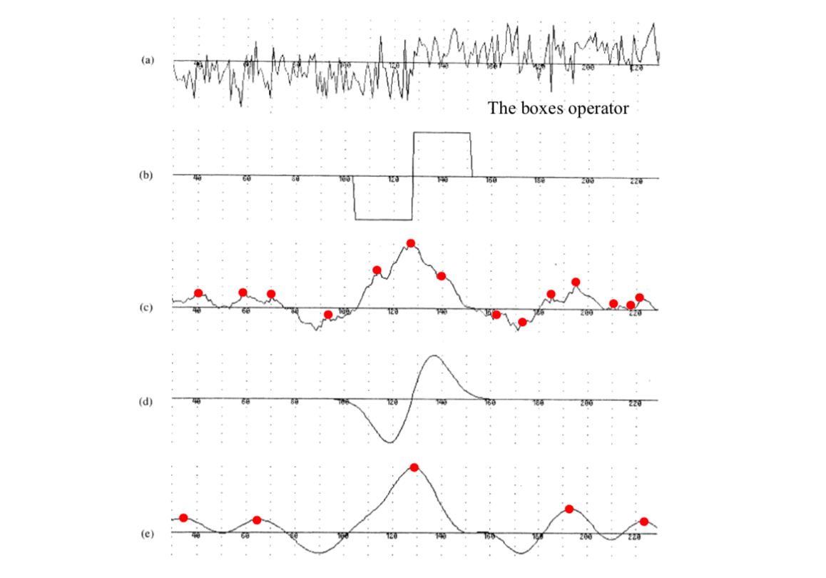
The edge center is marked as red circle at a local maximum in the output of the filter responses. Within the region of the edge, the boxes operator exhibits more local maxima than the Gaussian operator. Therefore, the Gaussian operator is better than the boxes operator in this example.
The three performance criteria
Good detection → Detection Criterion
There should be a low probability of failing to mark real edge points, and low probability of falsely marking non-edge points. This is controlled by signal-to-noise ratio: \[ \text{SNR}=\frac{|\int_{-w}^{+w}G(-x)f(x)dx |}{n_0\sqrt{\int_{-w}^{+w}f(x)^2dx}} \]
Good localization → Localization Criterion
The points marked as edge points by the operator should be as close as possible to the true edge center. The localization is defined as the reciprocal of \(\delta x_0\): \[ \text{Localization}=\frac{|\int_{-w}^{+w}G(-x)f'(x)dx |}{n_0\sqrt{\int_{-w}^{+w}f'(x)^2dx}} \]
Only one response to a single edge → Multiple Response Constraint \[ x_{zc}(f)=\pi\left(\frac{\int_{-\infty}^{+\infty}f'(x)^2dx}{\int_{-\infty}^{+\infty}f''(x)^2dx}\right)^{1/2} \]
It is very difficult to find the function \(f\) (filter) which maximizes the detection and localization criteria subject to the multiple response constraint. Numerical optimization is therefore used.
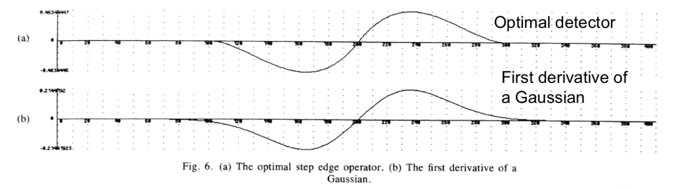
The solution is of the form \[ f(x)=a_1e^{\alpha x}\sin\omega x+a_2e^{\alpha x}\cos\omega x+a_3e^{-\alpha x}\sin\omega x\\ +a_4e^{-\alpha x}\cos\omega x+c \] The variables are determined by the non-linear optimization with boundary conditions.
The numerically estimated optimal edge detector can be approximated by the first derivative of a Gaussian G, where \[ G(x)=\exp(-\frac{x^2}{2\sigma^2})\\ f(x)=G'(x)=-\frac{x}{\sigma^2}\exp(-\frac{x^2}{2\sigma^2}) \] For 2D, the solution proposed by Canny amounts to convolving the initial image with a Gaussian function followed by computation of the derivatives in \(x\) and \(y\) of the result.
There are three main steps in the Canny edge detection
Gradient calculation
compute \(M\): \[ I_x=\frac{\partial}{\partial x}(I\ast G(x,y))\\ I_y=\frac{\partial}{\partial y}(I\ast G(x,y))\\ M=\sqrt{I_x^2+I_y^2}\approx |I_x|+|I_y| \]
Non-maximum suppression
keep local maximum, set others to zero.
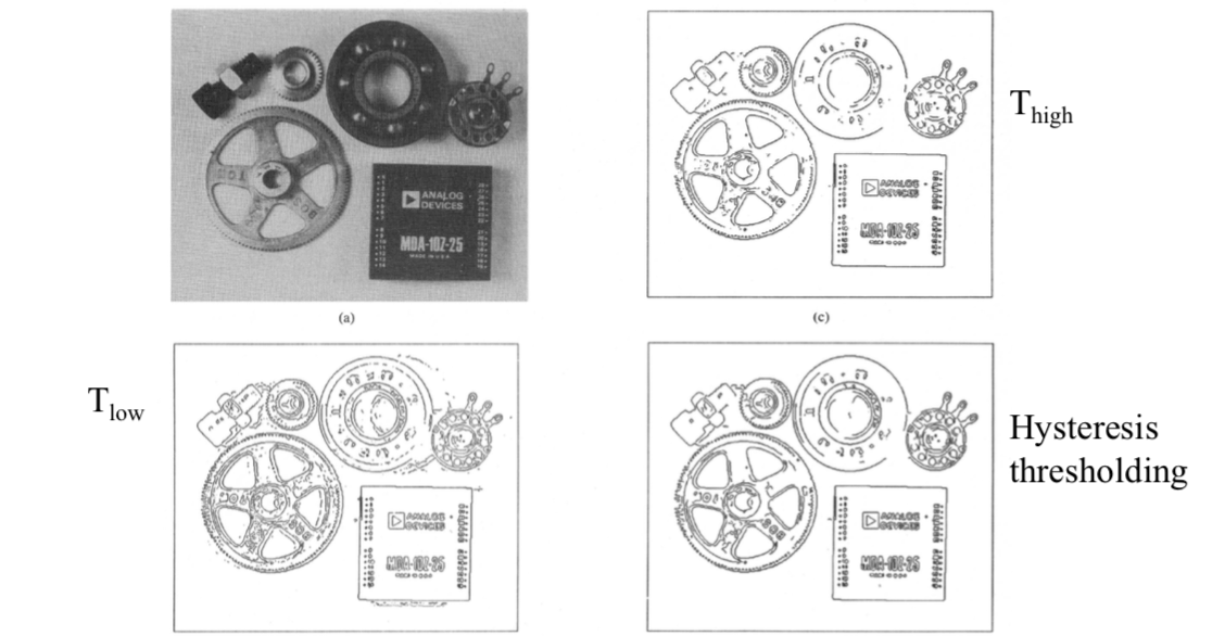
Hysteresis thresholding
Vehicle Detection based on Symmetry
Vehicle detection is based on the assumption that the rear or frontal views of the vehicles are generally symmetric; can be characterized by a rectangular bounding box which satisfies specific aspect ratio constraints and is placed in a specific region of the image, e.g., within lanes.
These features are used to identify vehicles in the image.
- Area of interest is identified on the basis of road position and perspective constraints.
- This area of interest is searched for possible vertical symmetries. Not only are the gray level symmetries considered, but also vertical and horizontal edge symmetries are considered.
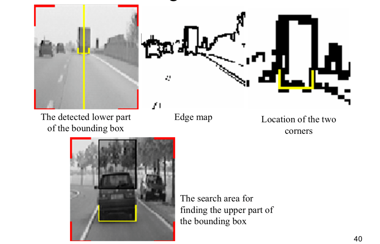
- Step 3: Once the symmetry axis has been detected, the lower part (the two bottom corners) of a rectangular bounding box is detected.
- The top horizontal limit of the vehicle is then searched according to the pre-defined aspect ratio.
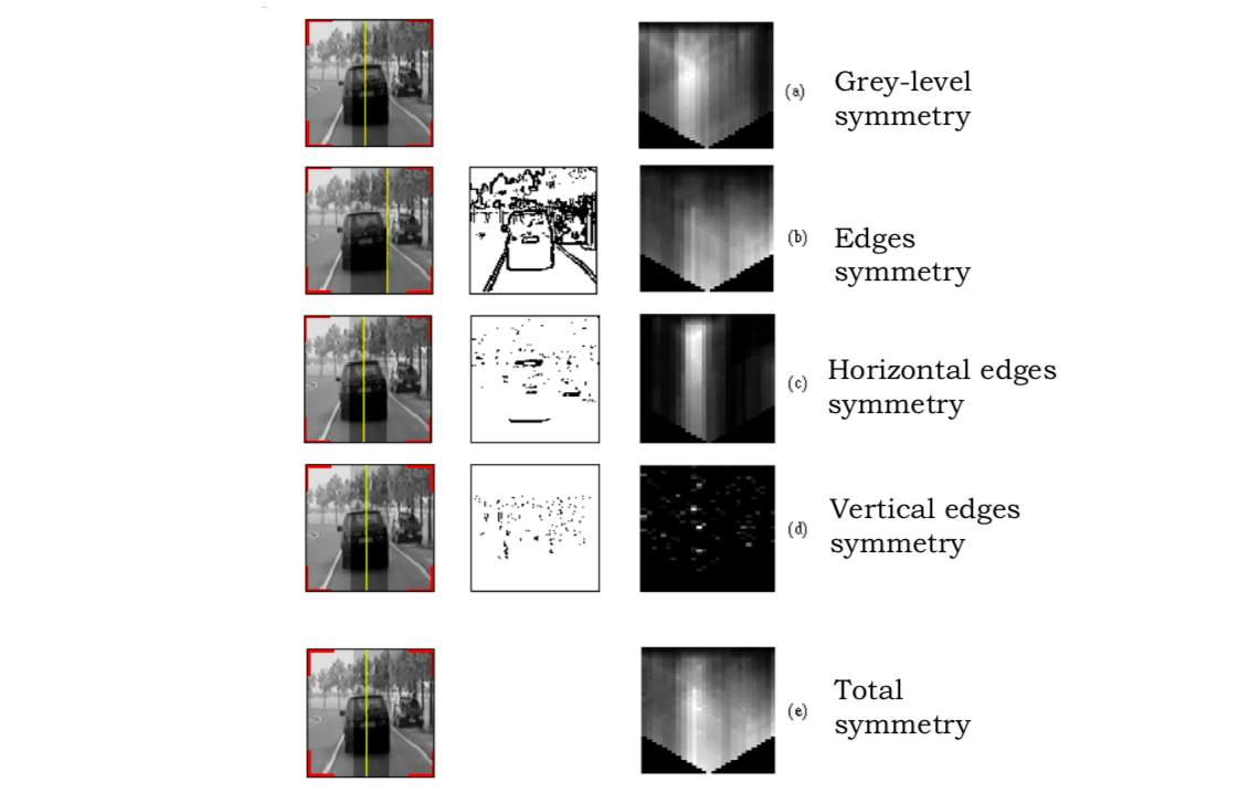
Vertical and horizontal binary edges can help solve the problems of strong reflection areas in the vehicle images. The analysis of symmetry produces symmetry maps for gray-level intensity, edge (total), horizontal edge, vertical edge and total (combined) symmetry. The symmetry axis can be found from the total symmetry map.
Bounding box detection
After detecting the symmetry axis, the width of the symmetrical region is checked for the presence of two corners representing the bottom of the bounding box around the vehicle.
Once the two corners are detected, the top side of the rectangle box can be detected by searching.
Visual Saliency For Detection and Tracking
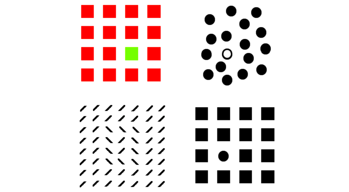
Visual saliency refers to the idea that certain parts of a scene are pre-attentively distinctive (pop-out) and create some form of immediate significant visual arousal within the early stages of the Human Visual System (HVS). The figure below is an example.
In image analysis, an edge is a pop-out region (region of saliency) since the edge is more visually significant than the other parts of the image.
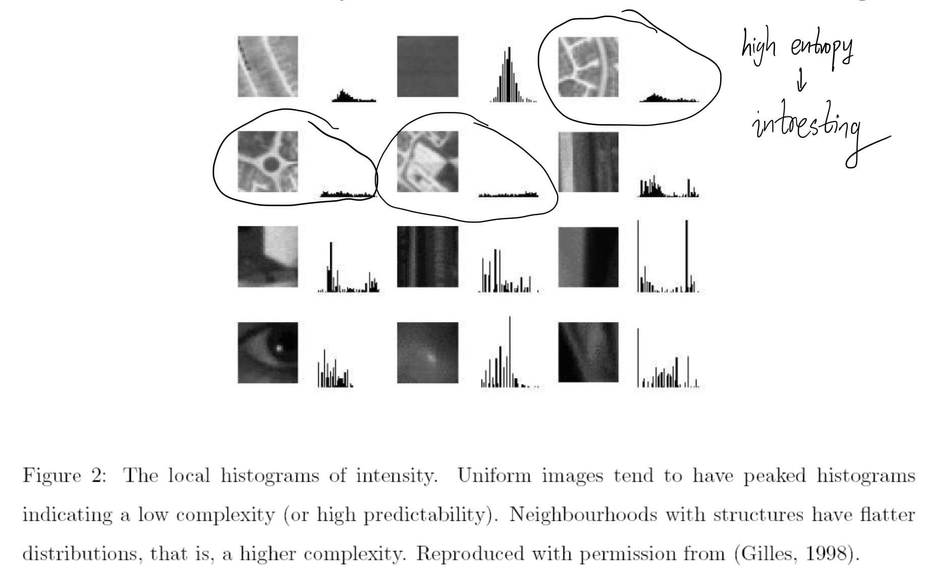
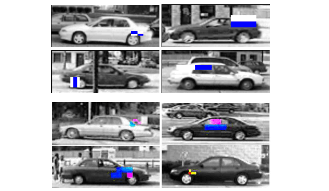
The salient points are literally the points on the object which are almost unique. These points maximize the discrimination between objects. The visual saliency is defined in terms of local signal complexity.
Shannon entropy of local attributes (called local entropy) is \[ H_{D,Rx}(x)=-\sum_{i\in D}P_{D,Rx}(x,d_i)\log_2P_{D,Rx}(x,d_i) \] where \(x\) is point location, \(Rx\) is local neighborhood at \(x\), \(D\) is descriptor (e.g. intensity), and \(P_{D,Rx}(x,d_i)\) is histogram value at \(x\).
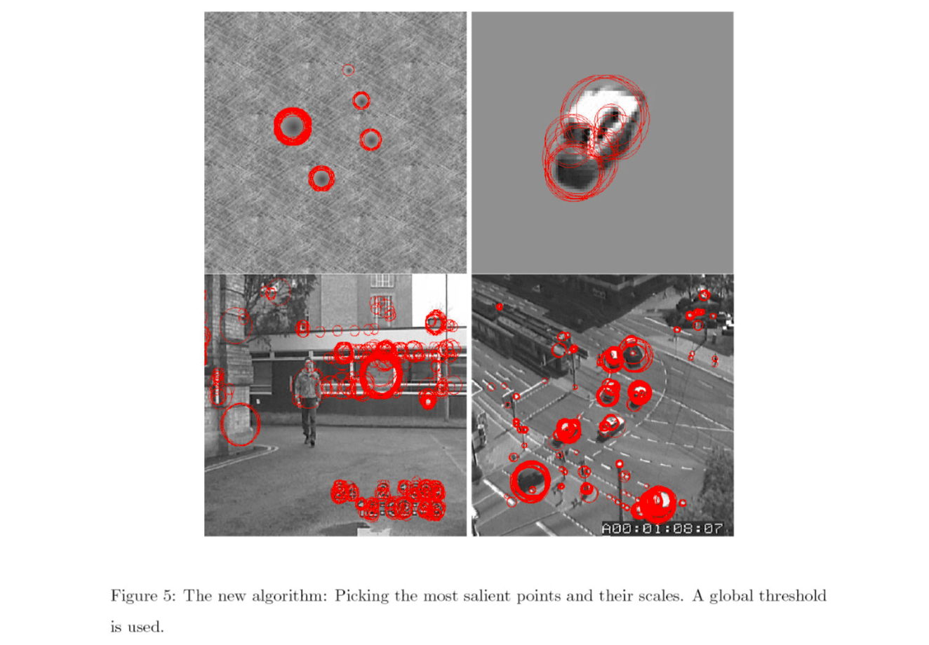
Below are sample frames from the processed sequences using a fixed scale based on local entropy. Red square boxes represent the most salient icons or parts of the image. The size of the local window or scale and threshold used were selected manually to give the most satisfactory results.
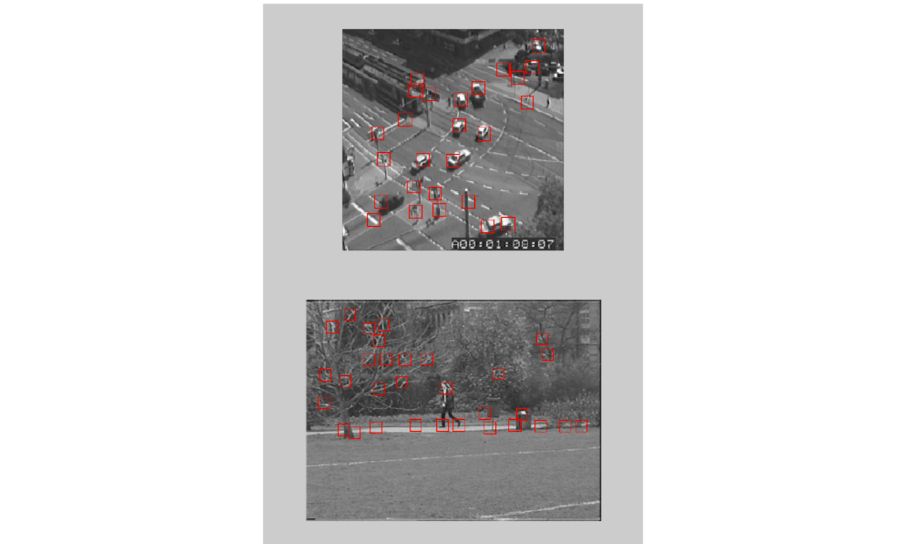
- Problem: the scale is fixed and global. For example, the scale is inappropriate for the pedestrians and the road markings in DT sequence.
- Problem: Small salient regions are not picked up. Highly textured regions, e.g., large intensity variation regions, are picked up. For example, trees and bushes in Vicky sequence.
Therefore, scale is an important and implicit part of the saliency detection problem.
Scale selection for salient region detection
Scale is selected based on the scale-space behavior of the saliency of a given feature.
For each pixel position \(x\)
For each scale \(s\) inside a range between \(s_\min\) and \(s_\max\) :
Measure the local descriptor values (e.g.,intensity values) within a window of scale \(s\).
Estimate the local probability density function (PDF) from this (e.g. using histogram).
Calculate the local entropy \(H_D\) \[ H_{D}(s,x)=-\sum_{i\in D}P_{D}(s,x,d_i)\log_2P_{D}(s,x,d_i) \]
Select scales for which the entropy is peaked \[ s:\frac{\partial^2H_D(s,x)}{\partial s^2}<0 \]
Detection performance can be further improved if change of histogram is considered.
Vehicle Detection by using AdaBoost
Vehicles can be detected by using AdaBoost.
By using the AdaBoost, vehicles in their lateral view can be detected in real time.
Vehicle Recognition
After vehicle detection, the vehicle can be recognition by using PCA and classification methods, e.g., k-NN or Bayesian methods.
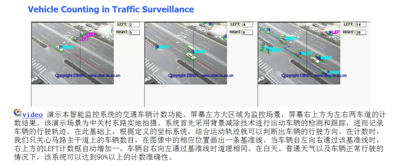
Application Examples
Vehicle counting in traffic surveillance
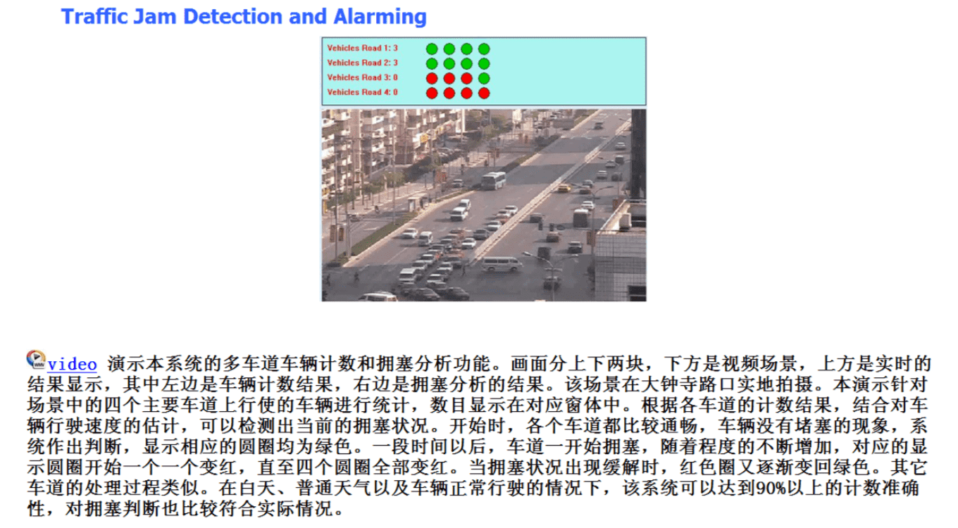
Traffic jam detection and alarming
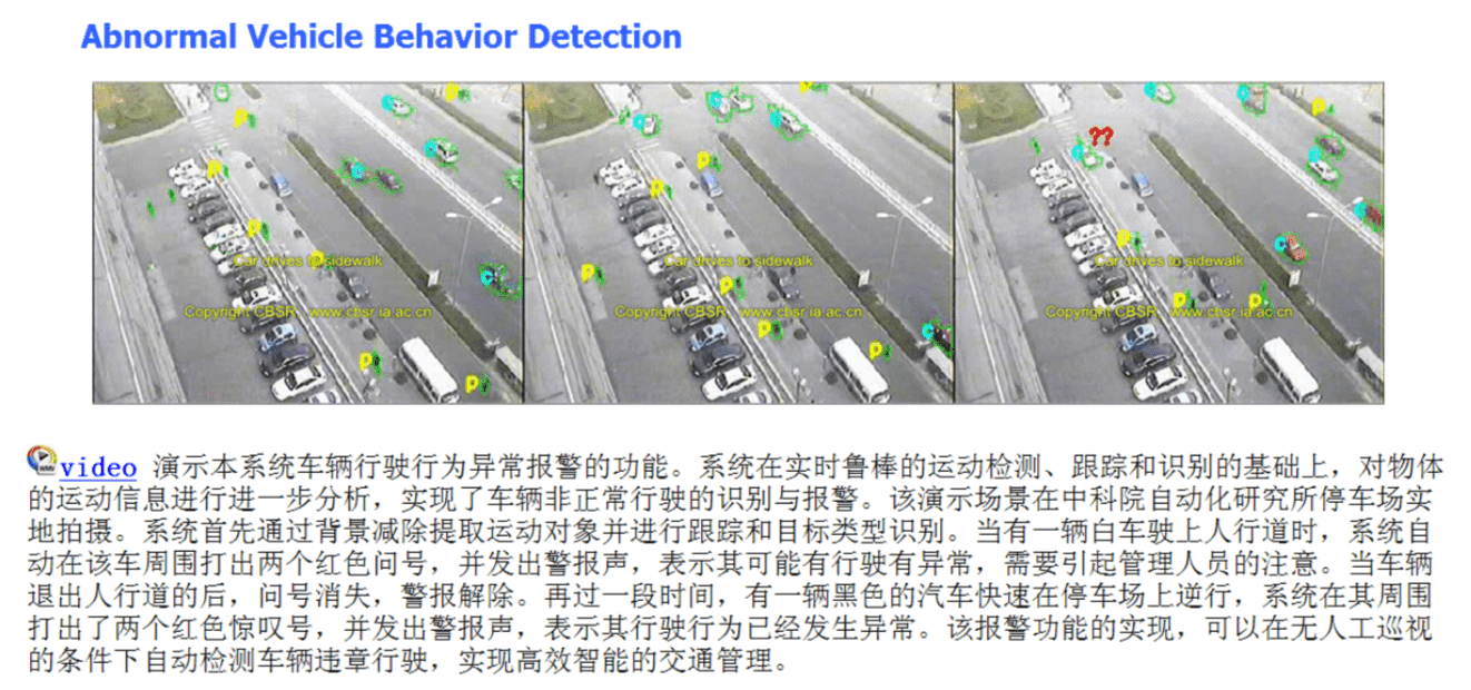
Abnormal vehicle behavior detection
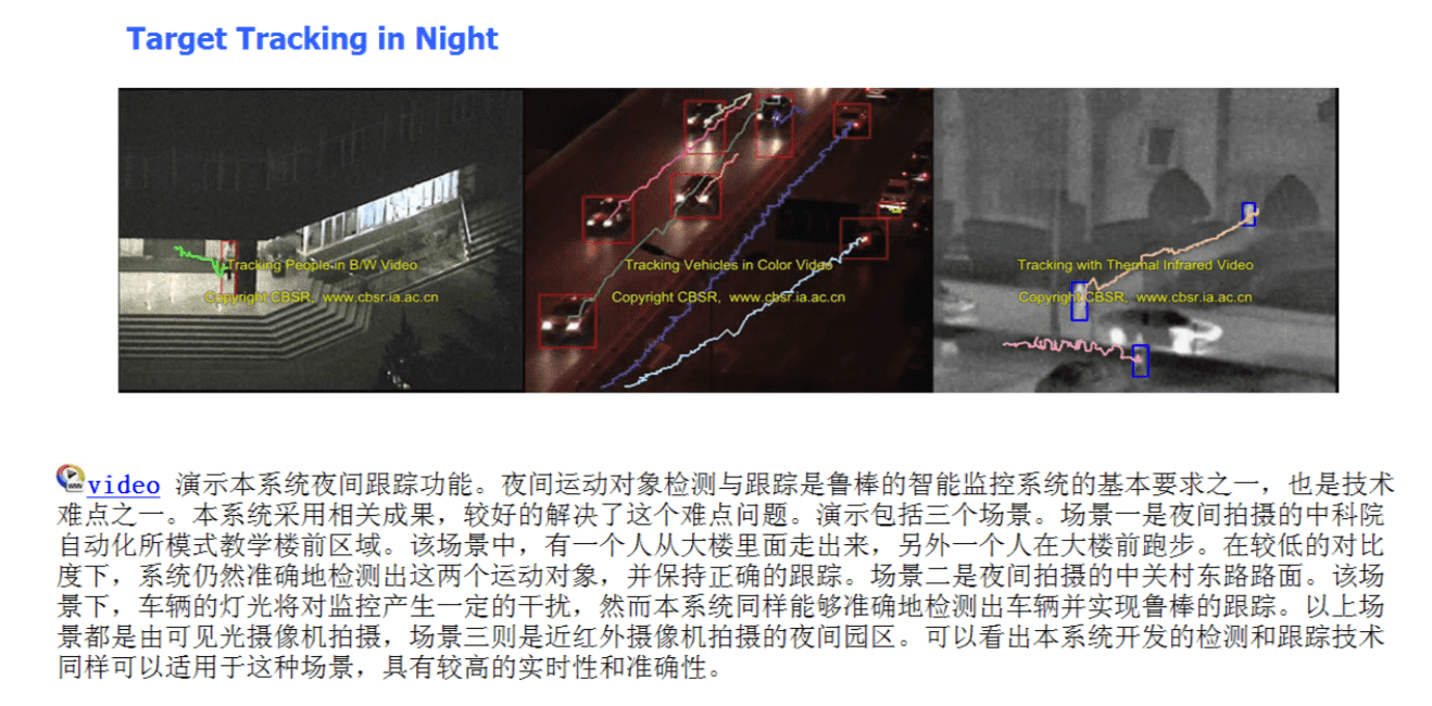
Target tracking in night